st558-project2
Predicting Popularity of Articles in the entertainment Channel
Claudia Donahue and Dane Korver 2022-06-28
Introduction
For this project, the dataset we are using summarizes a heterogeneous set of statistics about articles published by Mashable over a period of two years. The goal is to predict an article’s number of shares to social networks (its popularity). We wanted to look at the patterns in the articles that were shared. For example, is the timing of the article, the headline, and the article’s content all relevant in determining the number of times the article gets shared? What about whether an article had a polarizing title versus a generic non-polarizing title. Then, we wanted to find out whether the number of keywords associated with an article impacted the number of shares it received. Here are our findings for studying how to predict the number of shares in social networks (popularity).
Data
We’ll begin by reading in the data set and looking at how it’s structured.
data <- readr::read_csv(file = "OnlineNewsPopularity.csv",
                        show_col_types = FALSE
                        )
# Look at structure of data set
str(data)
## spec_tbl_df [39,644 × 61] (S3: spec_tbl_df/tbl_df/tbl/data.frame)
##  $ url                          : chr [1:39644] "http://mashable.com/2013/01/07/amazon-instant-video-browser/" "http://mashable.com/2013/01/07/ap-samsung-sponsored-tweets/" "http://mashable.com/2013/01/07/apple-40-billion-app-downloads/" "http://mashable.com/2013/01/07/astronaut-notre-dame-bcs/" ...
##  $ timedelta                    : num [1:39644] 731 731 731 731 731 731 731 731 731 731 ...
##  $ n_tokens_title               : num [1:39644] 12 9 9 9 13 10 8 12 11 10 ...
##  $ n_tokens_content             : num [1:39644] 219 255 211 531 1072 ...
##  $ n_unique_tokens              : num [1:39644] 0.664 0.605 0.575 0.504 0.416 ...
##  $ n_non_stop_words             : num [1:39644] 1 1 1 1 1 ...
##  $ n_non_stop_unique_tokens     : num [1:39644] 0.815 0.792 0.664 0.666 0.541 ...
##  $ num_hrefs                    : num [1:39644] 4 3 3 9 19 2 21 20 2 4 ...
##  $ num_self_hrefs               : num [1:39644] 2 1 1 0 19 2 20 20 0 1 ...
##  $ num_imgs                     : num [1:39644] 1 1 1 1 20 0 20 20 0 1 ...
##  $ num_videos                   : num [1:39644] 0 0 0 0 0 0 0 0 0 1 ...
##  $ average_token_length         : num [1:39644] 4.68 4.91 4.39 4.4 4.68 ...
##  $ num_keywords                 : num [1:39644] 5 4 6 7 7 9 10 9 7 5 ...
##  $ data_channel_is_lifestyle    : num [1:39644] 0 0 0 0 0 0 1 0 0 0 ...
##  $ data_channel_is_entertainment: num [1:39644] 1 0 0 1 0 0 0 0 0 0 ...
##  $ data_channel_is_bus          : num [1:39644] 0 1 1 0 0 0 0 0 0 0 ...
##  $ data_channel_is_socmed       : num [1:39644] 0 0 0 0 0 0 0 0 0 0 ...
##  $ data_channel_is_tech         : num [1:39644] 0 0 0 0 1 1 0 1 1 0 ...
##  $ data_channel_is_world        : num [1:39644] 0 0 0 0 0 0 0 0 0 1 ...
##  $ kw_min_min                   : num [1:39644] 0 0 0 0 0 0 0 0 0 0 ...
##  $ kw_max_min                   : num [1:39644] 0 0 0 0 0 0 0 0 0 0 ...
##  $ kw_avg_min                   : num [1:39644] 0 0 0 0 0 0 0 0 0 0 ...
##  $ kw_min_max                   : num [1:39644] 0 0 0 0 0 0 0 0 0 0 ...
##  $ kw_max_max                   : num [1:39644] 0 0 0 0 0 0 0 0 0 0 ...
##  $ kw_avg_max                   : num [1:39644] 0 0 0 0 0 0 0 0 0 0 ...
##  $ kw_min_avg                   : num [1:39644] 0 0 0 0 0 0 0 0 0 0 ...
##  $ kw_max_avg                   : num [1:39644] 0 0 0 0 0 0 0 0 0 0 ...
##  $ kw_avg_avg                   : num [1:39644] 0 0 0 0 0 0 0 0 0 0 ...
##  $ self_reference_min_shares    : num [1:39644] 496 0 918 0 545 8500 545 545 0 0 ...
##  $ self_reference_max_shares    : num [1:39644] 496 0 918 0 16000 8500 16000 16000 0 0 ...
##  $ self_reference_avg_sharess   : num [1:39644] 496 0 918 0 3151 ...
##  $ weekday_is_monday            : num [1:39644] 1 1 1 1 1 1 1 1 1 1 ...
##  $ weekday_is_tuesday           : num [1:39644] 0 0 0 0 0 0 0 0 0 0 ...
##  $ weekday_is_wednesday         : num [1:39644] 0 0 0 0 0 0 0 0 0 0 ...
##  $ weekday_is_thursday          : num [1:39644] 0 0 0 0 0 0 0 0 0 0 ...
##  $ weekday_is_friday            : num [1:39644] 0 0 0 0 0 0 0 0 0 0 ...
##  $ weekday_is_saturday          : num [1:39644] 0 0 0 0 0 0 0 0 0 0 ...
##  $ weekday_is_sunday            : num [1:39644] 0 0 0 0 0 0 0 0 0 0 ...
##  $ is_weekend                   : num [1:39644] 0 0 0 0 0 0 0 0 0 0 ...
##  $ LDA_00                       : num [1:39644] 0.5003 0.7998 0.2178 0.0286 0.0286 ...
##  $ LDA_01                       : num [1:39644] 0.3783 0.05 0.0333 0.4193 0.0288 ...
##  $ LDA_02                       : num [1:39644] 0.04 0.0501 0.0334 0.4947 0.0286 ...
##  $ LDA_03                       : num [1:39644] 0.0413 0.0501 0.0333 0.0289 0.0286 ...
##  $ LDA_04                       : num [1:39644] 0.0401 0.05 0.6822 0.0286 0.8854 ...
##  $ global_subjectivity          : num [1:39644] 0.522 0.341 0.702 0.43 0.514 ...
##  $ global_sentiment_polarity    : num [1:39644] 0.0926 0.1489 0.3233 0.1007 0.281 ...
##  $ global_rate_positive_words   : num [1:39644] 0.0457 0.0431 0.0569 0.0414 0.0746 ...
##  $ global_rate_negative_words   : num [1:39644] 0.0137 0.01569 0.00948 0.02072 0.01213 ...
##  $ rate_positive_words          : num [1:39644] 0.769 0.733 0.857 0.667 0.86 ...
##  $ rate_negative_words          : num [1:39644] 0.231 0.267 0.143 0.333 0.14 ...
##  $ avg_positive_polarity        : num [1:39644] 0.379 0.287 0.496 0.386 0.411 ...
##  $ min_positive_polarity        : num [1:39644] 0.1 0.0333 0.1 0.1364 0.0333 ...
##  $ max_positive_polarity        : num [1:39644] 0.7 0.7 1 0.8 1 0.6 1 1 0.8 0.5 ...
##  $ avg_negative_polarity        : num [1:39644] -0.35 -0.119 -0.467 -0.37 -0.22 ...
##  $ min_negative_polarity        : num [1:39644] -0.6 -0.125 -0.8 -0.6 -0.5 -0.4 -0.5 -0.5 -0.125 -0.5 ...
##  $ max_negative_polarity        : num [1:39644] -0.2 -0.1 -0.133 -0.167 -0.05 ...
##  $ title_subjectivity           : num [1:39644] 0.5 0 0 0 0.455 ...
##  $ title_sentiment_polarity     : num [1:39644] -0.188 0 0 0 0.136 ...
##  $ abs_title_subjectivity       : num [1:39644] 0 0.5 0.5 0.5 0.0455 ...
##  $ abs_title_sentiment_polarity : num [1:39644] 0.188 0 0 0 0.136 ...
##  $ shares                       : num [1:39644] 593 711 1500 1200 505 855 556 891 3600 710 ...
##  - attr(*, "spec")=
##   .. cols(
##   ..   url = col_character(),
##   ..   timedelta = col_double(),
##   ..   n_tokens_title = col_double(),
##   ..   n_tokens_content = col_double(),
##   ..   n_unique_tokens = col_double(),
##   ..   n_non_stop_words = col_double(),
##   ..   n_non_stop_unique_tokens = col_double(),
##   ..   num_hrefs = col_double(),
##   ..   num_self_hrefs = col_double(),
##   ..   num_imgs = col_double(),
##   ..   num_videos = col_double(),
##   ..   average_token_length = col_double(),
##   ..   num_keywords = col_double(),
##   ..   data_channel_is_lifestyle = col_double(),
##   ..   data_channel_is_entertainment = col_double(),
##   ..   data_channel_is_bus = col_double(),
##   ..   data_channel_is_socmed = col_double(),
##   ..   data_channel_is_tech = col_double(),
##   ..   data_channel_is_world = col_double(),
##   ..   kw_min_min = col_double(),
##   ..   kw_max_min = col_double(),
##   ..   kw_avg_min = col_double(),
##   ..   kw_min_max = col_double(),
##   ..   kw_max_max = col_double(),
##   ..   kw_avg_max = col_double(),
##   ..   kw_min_avg = col_double(),
##   ..   kw_max_avg = col_double(),
##   ..   kw_avg_avg = col_double(),
##   ..   self_reference_min_shares = col_double(),
##   ..   self_reference_max_shares = col_double(),
##   ..   self_reference_avg_sharess = col_double(),
##   ..   weekday_is_monday = col_double(),
##   ..   weekday_is_tuesday = col_double(),
##   ..   weekday_is_wednesday = col_double(),
##   ..   weekday_is_thursday = col_double(),
##   ..   weekday_is_friday = col_double(),
##   ..   weekday_is_saturday = col_double(),
##   ..   weekday_is_sunday = col_double(),
##   ..   is_weekend = col_double(),
##   ..   LDA_00 = col_double(),
##   ..   LDA_01 = col_double(),
##   ..   LDA_02 = col_double(),
##   ..   LDA_03 = col_double(),
##   ..   LDA_04 = col_double(),
##   ..   global_subjectivity = col_double(),
##   ..   global_sentiment_polarity = col_double(),
##   ..   global_rate_positive_words = col_double(),
##   ..   global_rate_negative_words = col_double(),
##   ..   rate_positive_words = col_double(),
##   ..   rate_negative_words = col_double(),
##   ..   avg_positive_polarity = col_double(),
##   ..   min_positive_polarity = col_double(),
##   ..   max_positive_polarity = col_double(),
##   ..   avg_negative_polarity = col_double(),
##   ..   min_negative_polarity = col_double(),
##   ..   max_negative_polarity = col_double(),
##   ..   title_subjectivity = col_double(),
##   ..   title_sentiment_polarity = col_double(),
##   ..   abs_title_subjectivity = col_double(),
##   ..   abs_title_sentiment_polarity = col_double(),
##   ..   shares = col_double()
##   .. )
##  - attr(*, "problems")=<externalptr>
# Checking to see whether the data has missing values
sum(is.na(data))
## [1] 0
The data has just one column that is not numeric, and that column is the
first one and contains URLs for the Mashable articles for each
observation. We will keep it, but won’t use it in our models. The second
column, timedelta, is not useful for prediction either. We will drop
this one. The other columns contain numeric data that we may be able to
use to predict the number of shares. The last column is our target
variable, shares. The data is set up nicely for what we want to do.
# Dropping the timedelta column

library(plyr)
library(tidyverse)
data <- select(data, -timedelta)

# Add a day column for data exploration/plotting purposes
data$day <- case_when(
  data$weekday_is_monday == 1 ~ "Monday",
  data$weekday_is_tuesday == 1 ~ "Tuesday",
  data$weekday_is_wednesday == 1 ~ "Wednesday",
  data$weekday_is_thursday == 1 ~ "Thursday",
  data$weekday_is_friday == 1 ~ "Friday",
  data$weekday_is_saturday == 1 ~ "Saturday",
  data$weekday_is_sunday == 1 ~ "Sunday"
)
data$day <- as_factor(data$day)

#Converting categorical values from numeric to factor - Weekdays
data$weekday_is_monday <- factor(data$weekday_is_monday)
data$weekday_is_tuesday <- factor(data$weekday_is_tuesday)
data$weekday_is_wednesday <- factor(data$weekday_is_wednesday)
data$weekday_is_thursday <- factor(data$weekday_is_thursday)
data$weekday_is_friday <- factor(data$weekday_is_friday)
data$weekday_is_saturday <- factor(data$weekday_is_saturday)
data$weekday_is_sunday <- factor(data$weekday_is_sunday)

# Add a channel column
data$chan <- case_when(
  data$data_channel_is_lifestyle == 1 ~ "Lifestyle",
  data$data_channel_is_entertainment == 1 ~ "Entertainment",
  data$data_channel_is_bus == 1 ~ "Business",
  data$data_channel_is_socmed == 1 ~ "Social Media",
  data$data_channel_is_tech == 1 ~ "Technology",
  data$data_channel_is_world == 1 ~ "World"
)
data$chan <- as_factor(data$chan)

#Converting categorical values from numeric to factor - News subjects
data$data_channel_is_lifestyle <- factor(data$data_channel_is_lifestyle)
data$data_channel_is_entertainment <- factor(data$data_channel_is_entertainment)
data$data_channel_is_bus <- factor(data$data_channel_is_bus)
data$data_channel_is_socmed <- factor(data$data_channel_is_socmed)
data$data_channel_is_tech <- factor(data$data_channel_is_tech)
data$data_channel_is_world <- factor(data$data_channel_is_world)
Next we will begin our look at one specific channel (entertainment) by subsetting the data.
channel <- channel # set = to channel when ready to automate

channelNow <- paste("data_channel_is_", channel, sep = "")

cData <- data[data[channelNow] == 1, ] # Extract rows of interest
We then split the entertainment channel’s data into training and testing
sets (70% and 30%, respectively). We will only explore the training set,
and will keep the testing set in reserve to determine the quality of our
predictions. We will use the function createDataPartition() from the
caret package to split the data.
library(caret) # Using createDataPartition from caret

set.seed(33) # for reproducibility

# Index to split on
idx <- createDataPartition(y = cData$shares, p = 0.7, list = FALSE)

# Subset
training <- cData[idx, ]
testing <- cData[-idx, ]
Summarizations
Then we thought about the characteristics of an online article that might be associated with someone deciding to “share” the article to someone else.
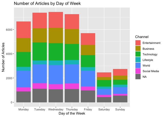
We thought it was probably important to consider both the timing of the article, the headline, and the article’s content. By timing, we mean that perhaps some readers are more likely to click on an article and share it on the weekend because they generally have more free time to read. But then we plotted the number of articles published each day, and realized not much gets published on the weekend, compared to weekdays. To visualize this pattern, we created the chart below:
ggplot(data) +
  geom_bar(aes(x = day, fill = chan)) +
  labs(title = "Number of Articles by Day of Week",
       x = "Day of the Week",
       y = "Number of Articles",
       fill = "Channel")
 A
table of the above chart:
A
table of the above chart:
data %>% group_by(day,chan) %>%
  summarise(n=n(),
            Avg=mean(shares),
            Sd=sd(shares),
            Median=median(shares),
            Min=min(shares),
            Max=max(shares))
## `summarise()` has grouped output by 'day'. You can override using the
## `.groups` argument.

## # A tibble: 49 × 8
## # Groups:   day [7]
##    day     chan              n   Avg     Sd Median   Min    Max
##    <fct>   <fct>         <int> <dbl>  <dbl>  <dbl> <dbl>  <dbl>
##  1 Monday  Entertainment  1358 2931.  7176.   1100    59 112600
##  2 Monday  Business       1153 3887. 28313.   1400     1 690400
##  3 Monday  Technology     1235 2821.  3915.   1600   192  51000
##  4 Monday  Lifestyle       322 4346. 14073.   1600   109 196700
##  5 Monday  World          1356 2456.  6865.   1100    43 141400
##  6 Monday  Social Media    337 4010.  6046.   2300    53  57600
##  7 Monday  <NA>            900 6961. 17388.   1900     4 200100
##  8 Tuesday Entertainment  1285 2708.  6453.   1100    47  98000
##  9 Tuesday Business       1182 2932. 10827.   1300    44 310800
## 10 Tuesday Technology     1474 2883.  4722.   1600   104  88500
## # … with 39 more rows
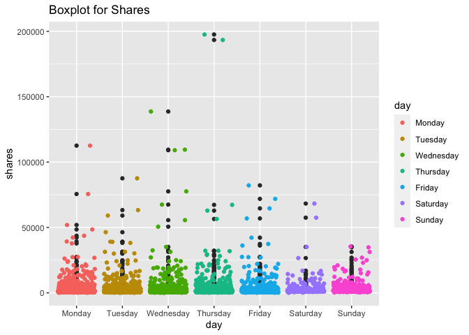
So we did away with that theory, and we will instead look at just the entertainment channel’s number of shares across days of the week.
ggplot(training, aes(x = day, y = shares)) +
  geom_boxplot() +
  geom_jitter(aes(color = day)) +
  ggtitle("Boxplot for Shares")
 A table of the above chart:
training %>% group_by(day,chan) %>%
  summarise(n=n(),
            Avg=mean(shares),
            Sd=sd(shares),
            Median=median(shares),
            Min=min(shares),
            Max=max(shares))
## `summarise()` has grouped output by 'day'. You can override using the
## `.groups` argument.

## # A tibble: 7 × 8
## # Groups:   day [7]
##   day       chan              n   Avg     Sd Median   Min    Max
##   <fct>     <fct>         <int> <dbl>  <dbl>  <dbl> <dbl>  <dbl>
## 1 Monday    Entertainment   949 2878.  6578.   1100    59 112600
## 2 Tuesday   Entertainment   901 2636.  5940.   1100    47  87600
## 3 Wednesday Entertainment   930 2915.  8649.   1100    49 138700
## 4 Thursday  Entertainment   852 3088. 10815.   1100    98 197600
## 5 Friday    Entertainment   674 2824.  6688.   1100    58  82200
## 6 Saturday  Entertainment   279 3251.  6311.   1600    65  68300
## 7 Sunday    Entertainment   356 3575.  4931.   1700   256  35400
The boxplot shows the distribution of the number of shares by the day of the week. It can be a good way to see if we have any outliers with way more shares than a typical article in this channel.
We wanted to look at these outliers–the entertainment channel’s top articles by shares, so we grabbed a list of those URLs, along with the number of shares.
head(training[order(training$shares, decreasing = TRUE), c("url", "shares")], 10)
## # A tibble: 10 × 2
##    url                                                                   shares
##    <chr>                                                                  <dbl>
##  1 http://mashable.com/2013/12/25/xbox-one-getting-started/              197600
##  2 http://mashable.com/2013/12/26/mcdonalds-kills-mcresource-line/       193400
##  3 http://mashable.com/2013/08/28/6000-video-launched-helloflo/          138700
##  4 http://mashable.com/2014/02/10/flappy-bird-typing-tutor/              112600
##  5 http://mashable.com/2014/10/14/sandworm-russian-hackers-nato-with-mi… 109500
##  6 http://mashable.com/2014/05/28/lookout-theft-protection/              109100
##  7 http://mashable.com/2014/11/23/employee-morale-holidays/               87600
##  8 http://mashable.com/2014/09/05/fall-activity-guide-seattle/            82200
##  9 http://mashable.com/2013/10/30/tesla-west-coast-free/                  77600
## 10 http://mashable.com/2014/03/31/google-plus-twitter-engagement/         75600
You can check out the article’s date and title within the URL and see what some of the most-shared articles were in the entertainment channel during the time period studied.
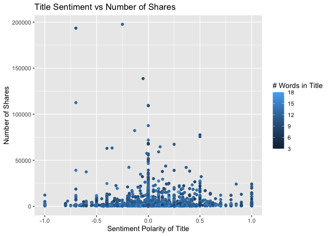
Then we wanted to create a visualization that would show us how the
variable title_sentiment_polarity seemed to impact the number of
shares. Our thought was that maybe an article with a more polarizing
title would get more shares than one less polarizing, as people want to
have some justification for urging a friend to spend time reading the
article. A polarizing sentiment could provide that justification for
some people. We will plot the polarity of the title’s sentiment and
include information on the number of words in the title.
ggplot(training, aes(x = title_sentiment_polarity,
                     y = shares,
                     color = n_tokens_title)) +
  geom_point() +
  labs(title = "Title Sentiment vs Number of Shares",
       x = "Sentiment Polarity of Title",
       y = "Number of Shares",
       color = "# Words in Title")
 A table of the above chart:
training %>% group_by(title_sentiment_polarity) %>%
  summarise(n=n(),
            Avg=mean(shares),
            Sd=sd(shares),
            Median=median(shares),
            Min=min(shares),
            Max=max(shares))
## # A tibble: 326 × 7
##    title_sentiment_polarity     n    Avg     Sd Median   Min    Max
##                       <dbl> <int>  <dbl>  <dbl>  <dbl> <dbl>  <dbl>
##  1                   -1        24  2152.  2427.   1300   556  12200
##  2                   -0.8       6  1560.   932.   1150   741   3100
##  3                   -0.78      1  5600     NA    5600  5600   5600
##  4                   -0.75      2   745    361.    745   490   1000
##  5                   -0.714     2   868    140.    868   769    967
##  6                   -0.7      27 15511. 41986.   1100   366 193400
##  7                   -0.667     1   911     NA     911   911    911
##  8                   -0.65      4  1221.   635.   1100   583   2100
##  9                   -0.638     1   855     NA     855   855    855
## 10                   -0.625    14  1432.  1156.    973   661   4900
## # … with 316 more rows
In this plot of the impact of the title’s sentiment polarity on shares, an upward trend in the plotted points would indicate that articles with higher values of title sentiment polarity tend to be shared more often. Note that polarity values can be positive or negative.
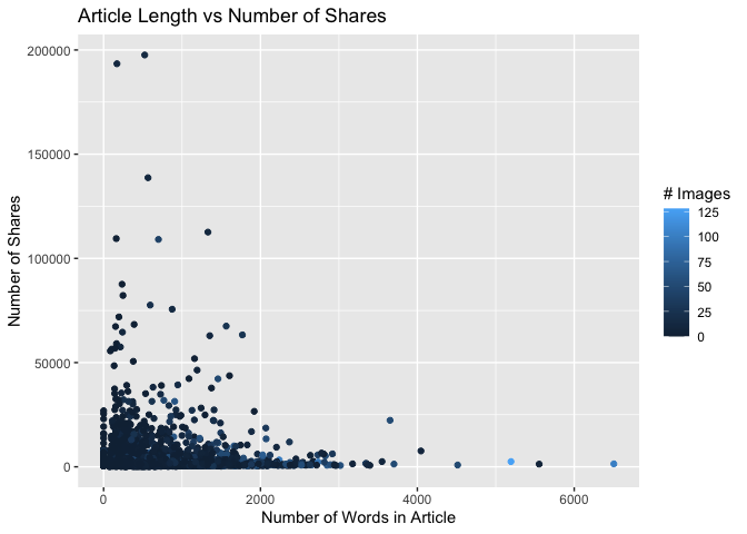
Finally, we thought about how the content of an article might lead someone to share it. Maybe people share shorter articles more than long ones. Maybe people like to share links with images more than links without images, we thought. So we took a look at an article’s length and number of images vs. number of shares.
ggplot(training, aes(x = n_tokens_content,
                     y = shares,
                     color = num_imgs)) +
  geom_point() +
  labs(title = "Article Length vs Number of Shares",
       x = "Number of Words in Article",
       y = "Number of Shares",
       color = "# Images")
 A table of the above chart:
training %>% group_by(n_tokens_content) %>%
  summarise(n=n(),
            Avg=mean(shares),
            Sd=sd(shares),
            Median=median(shares),
            Min=min(shares),
            Max=max(shares))
## # A tibble: 1,499 × 7
##    n_tokens_content     n   Avg    Sd Median   Min   Max
##               <dbl> <int> <dbl> <dbl>  <dbl> <dbl> <dbl>
##  1                0   145 2886. 4466.  1200    379 26900
##  2               43     1  860    NA    860    860   860
##  3               53     1 1200    NA   1200   1200  1200
##  4               54     1 1600    NA   1600   1600  1600
##  5               55     1  711    NA    711    711   711
##  6               58     1 2000    NA   2000   2000  2000
##  7               66     1 7800    NA   7800   7800  7800
##  8               73     2  654.  771.   654.   109  1200
##  9               76     1  630    NA    630    630   630
## 10               77     1 3800    NA   3800   3800  3800
## # … with 1,489 more rows
In this plot, a downward trend in plotted points would indicate that shorter articles generally get more shares, while an upward trend would indicate that longer articles achieve more shares.
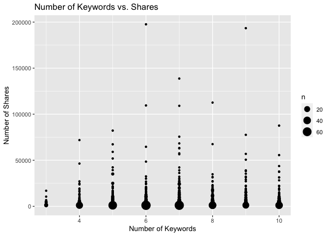
Next we looked at an article’s keyword characteristics. Within its metadata, a website can be assigned a number of keywords, which used to give search engines more information about the content. We wondered how the number of keywords related to the number of shares, given that this data is several years old, and that used to be considered a part of search engine optimization.
ggplot(training, aes(x = num_keywords,
                     y = shares)) +
  geom_count() +
  labs(title = "Number of Keywords vs. Shares",
       x = "Number of Keywords",
       y = "Number of Shares")
 A table of the above chart:
training %>% group_by(num_keywords) %>%
  summarise(n=n(),
            Avg=mean(shares),
            Sd=sd(shares),
            Median=median(shares),
            Min=min(shares),
            Max=max(shares))
## # A tibble: 8 × 7
##   num_keywords     n   Avg     Sd Median   Min    Max
##          <dbl> <int> <dbl>  <dbl>  <dbl> <dbl>  <dbl>
## 1            3    64 1950.  2581.   1100   478  16900
## 2            4   454 2148.  4955.   1000    50  71900
## 3            5   769 2684.  6205.   1100    58  82200
## 4            6   940 2722.  8480.   1100    49 197600
## 5            7   878 3472.  9094.   1200   109 138700
## 6            8   673 2968.  6498.   1200    88 112600
## 7            9   481 3863. 11134.   1300    47 193400
## 8           10   682 2793.  5651.   1300    80  87600
The plot depicts circles sized by the number of articles falling into that category of number of keywords and number of shares. So you can how many keywords are typically used, and also whether any specific number of keywords tends to achieve more shares.
Before the modeling step, we took one final look at a few more of the other variables we thought might be important in predicting number of shares, based on the summaries above and our own experiences.
library(GGally)
training %>%
  select(self_reference_avg_sharess, LDA_00, rate_negative_words, shares) %>%
  GGally::ggpairs()
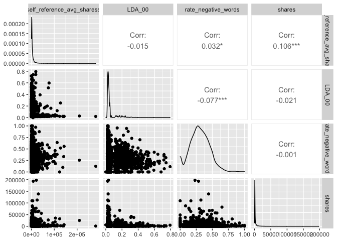
Looking across the bottom row of graphs, we can see whether any
relationships between shares and another variable are evident.
Modeling
Now we were ready to create some predictive models using the training data.
Linear Regression
Linear regression is a way of calculating the relationship between one
or more input/independent variables and an output/dependent variable.
(More than one input variable would make the model a multiple
regression) In this case, our output variables is shares, the number
of times a Mashable article was shared. A linear regression assumes that
one or more other variables are correlated with the number of shares,
and that the relationship can be visually represented as a straight
line. The mathematical equation for a basic linear regression is:
where y is the dependent variable, x is an independent variable, and A and B are coefficients for the line’s y-intercept and slope. The values for these coefficients are chosen to minimize the error between the model’s predictions and the actual outcomes in the training data.
With that, here we go! We are using the train() function from the
caret package to make the model. We will use the results of 5-fold
cross-validation to evaluate the performance of all our models and,
later, to compare them.
This first multiple regression (linear regression model extended to include more explanatory variables and/or higher order terms) will try to predict the number of shares based on most of the available data in our training dataset.
# building the model
fullFit <- train(shares ~ n_tokens_content + num_hrefs + num_self_hrefs +
                     average_token_length + num_keywords +
                     kw_min_max + kw_max_max + kw_avg_max + kw_max_avg +
                     kw_avg_avg + self_reference_min_shares + weekday_is_monday +
                     weekday_is_tuesday + weekday_is_wednesday +
                     weekday_is_thursday + weekday_is_friday +
                     global_subjectivity + title_sentiment_polarity,
              data = training,
              method = "lm", # linear regression
              preProcess = c("center", "scale", "nzv"),
              trControl = trainControl(method = "cv", number = 2)
              )
# look at the resulting coefficients
fullFit$finalModel
##
## Call:
## lm(formula = .outcome ~ ., data = dat)
##
## Coefficients:
##               (Intercept)           n_tokens_content
##                   2941.05                    -163.15
##                 num_hrefs             num_self_hrefs
##                    548.39                    -180.28
##      average_token_length               num_keywords
##                    -13.10                     -33.01
##                kw_max_max                 kw_avg_max
##                    -80.14                    -253.49
##                kw_max_avg                 kw_avg_avg
##                    416.77                    1418.83
## self_reference_min_shares         weekday_is_monday1
##                    441.37                    -210.31
##       weekday_is_tuesday1      weekday_is_wednesday1
##                   -280.13                    -135.36
##      weekday_is_thursday1         weekday_is_friday1
##                   -127.44                    -168.98
##       global_subjectivity   title_sentiment_polarity
##                    259.18                    -143.50
fullFit
## Linear Regression
##
## 4941 samples
##   18 predictor
##
## Pre-processing: centered (17), scaled (17), remove (1)
## Resampling: Cross-Validated (2 fold)
## Summary of sample sizes: 2470, 2471
## Resampling results:
##
##   RMSE    Rsquared    MAE
##   7675.5  0.02772562  2922.109
##
## Tuning parameter 'intercept' was held constant at a value of TRUE
The next multiple regresson model is a little more simplified and includes a smaller subset of variables that we think would be important.
smallFit <- train(shares ~ n_tokens_content + num_hrefs + num_self_hrefs +
                     average_token_length + num_keywords +
                     kw_min_max + kw_max_max + kw_avg_max + kw_max_avg +
                     kw_avg_avg + self_reference_min_shares +
                     global_subjectivity + title_sentiment_polarity,
              data = training,
              method = "lm",
              preProcess = c("center", "scale", "nzv"),
              trControl = trainControl(method = "cv", number = 2)
              )
# look at the resulting coefficients
smallFit$finalModel
##
## Call:
## lm(formula = .outcome ~ ., data = dat)
##
## Coefficients:
##               (Intercept)           n_tokens_content
##                  2941.046                   -149.345
##                 num_hrefs             num_self_hrefs
##                   544.520                   -185.028
##      average_token_length               num_keywords
##                    -6.769                    -13.864
##                kw_max_max                 kw_avg_max
##                   -89.308                   -247.650
##                kw_max_avg                 kw_avg_avg
##                   406.873                   1428.439
## self_reference_min_shares        global_subjectivity
##                   441.518                    255.390
##  title_sentiment_polarity
##                  -147.249
smallFit
## Linear Regression
##
## 4941 samples
##   13 predictor
##
## Pre-processing: centered (12), scaled (12), remove (1)
## Resampling: Cross-Validated (2 fold)
## Summary of sample sizes: 2471, 2470
## Resampling results:
##
##   RMSE      Rsquared    MAE
##   7703.519  0.03210185  2916.344
##
## Tuning parameter 'intercept' was held constant at a value of TRUE
Random Forest
Random forest is a tree-based method of prediction. It does not use all predictors available, but instead uses a random subset of predictors for each of many bootstrap samples / tree fits.
# load required package
library(randomForest)
# set up the mtry parameter
tunegrid <- expand.grid(.mtry=c(1:3)) # This is key for amount of time running

#train model
rfFit <- train(x = select(training, -url, -shares, -day, -chan),
                y = training$shares,
                method = "rf",
                tuneGrid = tunegrid,
                preProcess = c("center", "scale", "nzv"),
                trControl = trainControl(method = "cv",
                                         number = 2)
                )
rfFit
## Random Forest
##
## 4941 samples
##   58 predictor
##
## Pre-processing: centered (44), scaled (44), ignore (13), remove (1)
## Resampling: Cross-Validated (2 fold)
## Summary of sample sizes: 2471, 2470
## Resampling results across tuning parameters:
##
##   mtry  RMSE      Rsquared    MAE
##   1     7619.296  0.01959718  2852.968
##   2     7590.858  0.02431664  2895.366
##   3     7591.657  0.02591852  2934.611
##
## RMSE was used to select the optimal model using the smallest value.
## The final value used for the model was mtry = 2.
Boosted Tree
Boosted tree models is another tree-based method of prediction. Although, unlike random forest models, boosted tree models grow sequentially with each subsequent grown on a modified version of the original data and the predictions updated as trees grow.
# Load required packages
library(gbm)

# set up the parameters
gbmGrid <-  expand.grid(interaction.depth = c(1, 2, 3),
                        n.trees = c(25, 50),
                        shrinkage = 0.1,
                        n.minobsinnode = 10)

#train model
btFit <- train(x = select(training, -url, -shares, -day, -chan),
                y = training$shares,
                method = "gbm",
                tuneGrid = gbmGrid,
                preProcess = c("center", "scale", "nzv"),
                trControl = trainControl(method = "cv",
                                         number = 2)
                )
## Iter   TrainDeviance   ValidDeviance   StepSize   Improve
##      1 69708909.4118             nan     0.1000 25698.3251
##      2 69285569.9168             nan     0.1000 -100419.1499
##      3 68401036.4675             nan     0.1000 802981.9801
##      4 68083848.2802             nan     0.1000 1554.4521
##      5 67358279.0681             nan     0.1000 516605.5073
##      6 66460383.0137             nan     0.1000 -89998.7333
##      7 66322587.5925             nan     0.1000 116610.8502
##      8 65693748.3397             nan     0.1000 -240432.2954
##      9 65361524.3274             nan     0.1000 1576.0785
##     10 65043937.1400             nan     0.1000 -184821.2171
##     20 62900443.6589             nan     0.1000 -135588.5157
##     40 61523012.4949             nan     0.1000 -164702.0894
##     50 61066773.9647             nan     0.1000 -313279.0538
##
## Iter   TrainDeviance   ValidDeviance   StepSize   Improve
##      1 68632543.2604             nan     0.1000 463919.5708
##      2 68246652.0941             nan     0.1000 97235.9687
##      3 67156422.4834             nan     0.1000 176859.3986
##      4 66719854.1553             nan     0.1000 44669.8595
##      5 65862976.7920             nan     0.1000 -413008.0917
##      6 65502268.1883             nan     0.1000 9965.4498
##      7 64860344.0939             nan     0.1000 -646443.9751
##      8 64630279.4233             nan     0.1000 -131488.6831
##      9 64422063.3921             nan     0.1000 152391.3072
##     10 64221101.0486             nan     0.1000 -158310.9917
##     20 60180290.3151             nan     0.1000 -142846.1885
##     40 56614294.1111             nan     0.1000 -71672.9699
##     50 54919678.6548             nan     0.1000 -93783.0503
##
## Iter   TrainDeviance   ValidDeviance   StepSize   Improve
##      1 69428505.7457             nan     0.1000 -108381.3574
##      2 68965514.0816             nan     0.1000 108691.6371
##      3 68115601.1883             nan     0.1000 556372.3988
##      4 67601868.4631             nan     0.1000 205104.9245
##      5 66382718.0345             nan     0.1000 -56128.9015
##      6 65905174.8338             nan     0.1000 164147.8012
##      7 64884165.2852             nan     0.1000 -284054.2288
##      8 64475815.6843             nan     0.1000 336617.6865
##      9 63976561.4396             nan     0.1000 -21082.4289
##     10 63870354.2288             nan     0.1000 -173117.7245
##     20 59657378.4388             nan     0.1000 -323109.9996
##     40 55006158.7523             nan     0.1000 -429462.3809
##     50 53926354.8890             nan     0.1000 -210950.2250
##
## Iter   TrainDeviance   ValidDeviance   StepSize   Improve
##      1 47805528.7224             nan     0.1000 87861.9114
##      2 47581394.7048             nan     0.1000 177905.9312
##      3 47423541.4588             nan     0.1000 30090.9287
##      4 47314595.1080             nan     0.1000 61972.6439
##      5 47104508.5096             nan     0.1000 114225.9636
##      6 46986549.5682             nan     0.1000 123860.5768
##      7 46823916.8082             nan     0.1000 105711.5188
##      8 46750527.9642             nan     0.1000 -45117.6583
##      9 46618455.2155             nan     0.1000 -15488.9615
##     10 46521573.4329             nan     0.1000 -55399.4911
##     20 45669083.8332             nan     0.1000 -20584.9134
##     40 44707105.4863             nan     0.1000 -55922.9180
##     50 44490269.1269             nan     0.1000 -88170.3752
##
## Iter   TrainDeviance   ValidDeviance   StepSize   Improve
##      1 47728020.7165             nan     0.1000 84543.6567
##      2 47523971.2853             nan     0.1000 -40639.7119
##      3 47356140.1595             nan     0.1000 -16191.8904
##      4 46870646.7184             nan     0.1000 -80420.5618
##      5 46639351.5310             nan     0.1000 -63942.3365
##      6 46225113.2850             nan     0.1000 45643.1938
##      7 45987549.6006             nan     0.1000 128700.2182
##      8 45561546.9256             nan     0.1000 142931.1586
##      9 45409468.1513             nan     0.1000 63923.6106
##     10 45156786.8497             nan     0.1000 -77683.4672
##     20 43727633.4437             nan     0.1000 9785.7781
##     40 41335290.4600             nan     0.1000 -96464.1906
##     50 40476978.9912             nan     0.1000 -103134.8391
##
## Iter   TrainDeviance   ValidDeviance   StepSize   Improve
##      1 47484173.2652             nan     0.1000 158482.8268
##      2 47054630.0173             nan     0.1000 29190.4764
##      3 46500497.9127             nan     0.1000 42888.8500
##      4 46124832.3511             nan     0.1000 -42360.8517
##      5 45843169.6825             nan     0.1000 -27354.0329
##      6 45389356.5151             nan     0.1000 71806.6591
##      7 45158274.1185             nan     0.1000 -86040.0680
##      8 44822830.5785             nan     0.1000 -58317.2241
##      9 44324221.4952             nan     0.1000 386992.0026
##     10 44161890.1819             nan     0.1000 -96930.0601
##     20 41750060.2056             nan     0.1000 -134751.8694
##     40 39101093.5544             nan     0.1000 -155986.5751
##     50 37635610.3755             nan     0.1000 -259726.9592
##
## Iter   TrainDeviance   ValidDeviance   StepSize   Improve
##      1 58441729.1014             nan     0.1000 63482.9145
##      2 57696620.8892             nan     0.1000 111086.4811
##      3 56967890.0007             nan     0.1000 126515.1968
##      4 56380462.9620             nan     0.1000 117757.6814
##      5 55885591.5636             nan     0.1000 82079.4144
##      6 54933130.3416             nan     0.1000 47171.5724
##      7 54593724.7993             nan     0.1000 -67175.2256
##      8 54369158.1788             nan     0.1000 -21282.6413
##      9 54221427.8766             nan     0.1000 -53698.1596
##     10 53923155.2964             nan     0.1000 -152461.6257
##     20 51752373.3043             nan     0.1000 -13761.2055
##     25 51413644.2548             nan     0.1000 -180239.8396
Comparison
We compared all four of these models using the test dataset.
# full fit multiple regression model
fullPred <- predict(fullFit, newdata = testing)
# selected variable multiple regression model
smallPred <- predict(smallFit, newdata = testing)
# random forest
rfPred <- predict(rfFit, newdata = testing)
# boosted tree
btPred <- predict(btFit, newdata = testing)
Now we will compare the four candidate models and choose one “winner”:
# Create a named with results (Rsquared values) for each model
results <- c("Full Fit" = max(fullFit$results$Rsquared),
           "Small Fit" = max(smallFit$results$Rsquared),
           "Random Forest" = max(rfFit$results$Rsquared),
           "Boosted Tree" = max(btFit$results$Rsquared))

# RSquared Values are:
results
##      Full Fit     Small Fit Random Forest  Boosted Tree
##    0.02772562    0.03210185    0.02591852    0.01723738
# The best model based on the highest R-squared value is:
winner <- results[which.max(results)]
winner
##  Small Fit
## 0.03210185
Above is our winning model for the entertainment channel based on it having the highest R-Squared value of 0.0321019! Our models are not doing that great, and only explain a small percentage of the variation in number of shares, but let’s not let that dampen our enthusiasm!
If we wanted to improve upon these models, we could increase the tuning
value of mtry in the Random Forest model. The cost would be the model
would take a lot longer to train. We also considered trying to predict
the
instead of
shares itself, but decided that was outside the scope of
the assignment.
Automation
We generated these reports automatically for each channel (“lifestyle”,
“entertainment”, “bus”, “socmed”, “tech”, and “world”) by creating a
function that uses the rmarkdown package to render a Github document
with a params option, and then using a for loop to execute that
function for each channel in a list. That’s how the entertainment
channel page you’re reading was generated!
The code we used to automate the rendering is visible at the main page for this project here.